Rainfall Seasonality as a
Multivariate Object

Bringing Biplots to life with moveEZ

Raeesa Ganey

3 September 2026

Two goals

1. A substantive question

Has rainfall seasonality in South Africa changed over the last three decades, and does the answer look different when the components are treated jointly rather than one at a time?

2. A methodological one

moveEZ is a new package for animated biplots. This is its first full application to a real climate panel, and the application exposes what the package can and cannot yet do.

The two are entangled on purpose. The climate problem motivated the diagnostics, and the diagnostics changed what could be claimed about the climate.

1. The univariate analysis

The starting point

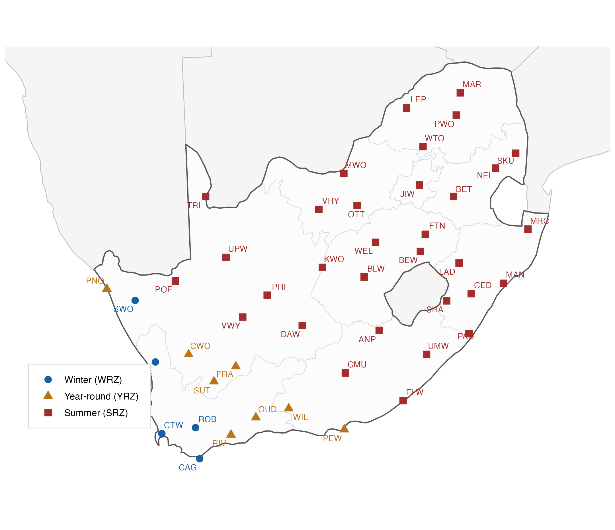
Roffe, Fitchett & Curtis (2021). Investigating changes in rainfall seasonality across South Africa.

• 46 rain gauge stations, chosen for record completeness
• 1987 to 2016, thirty accumulation years
• Stations classified into winter (WRZ), summer (SRZ) and year-round (YRZ) rainfall zones

The seven components

Component	Definition
start	onset day of the wet season
end	cessation day
length	duration of the wet season
total	wet-season rainfall accumulation
raindays	number of rain days
rate	mean rainfall per rain day
score	rainfall:temperature seasonality index

The score contrasts summer against winter rainfall relative to the temperature cycle. Negative values indicate winter-rainfall conditions.

What was done with them

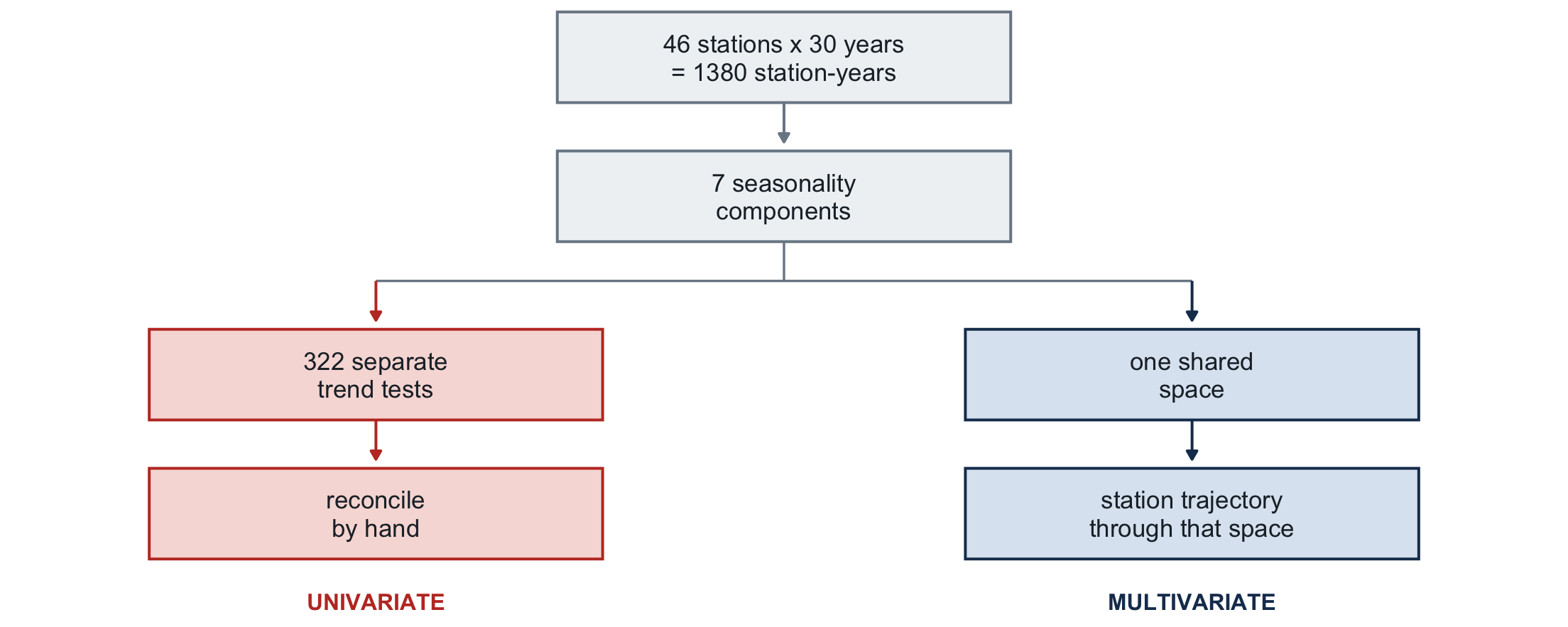
For each station, for each component, a trend is fitted across the thirty years and tested for significance.

\[46 \text{ stations} \times 7 \text{ components} = \mathbf{322} \text{ univariate trend tests}\]

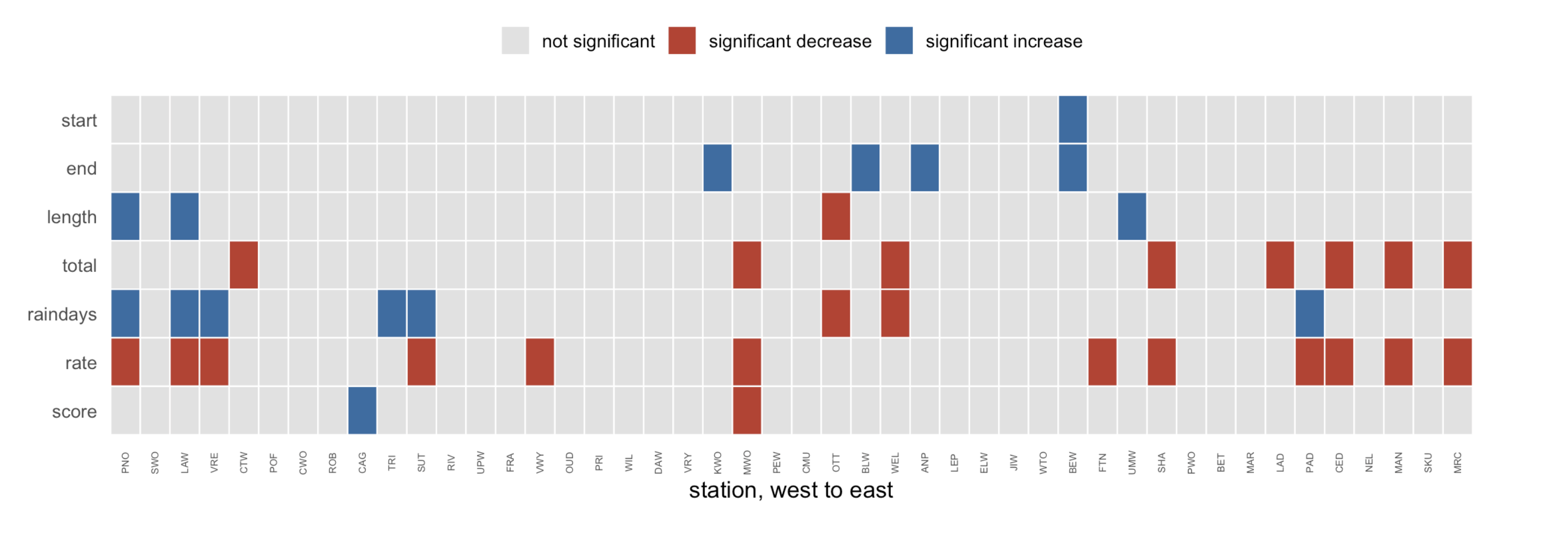
39 significant trends detected.

What they found

• Winter-rainfall stations in the southwestern Cape and along the west coast trending towards more evenly distributed rainfall, scores tending towards zero
• Southern-coast stations moving the other way: Oudtshoorn, Port Elizabeth, Riversdale, Robertson, towards stronger winter-rainfall conditions
• Later start dates across much of the interior
• Eight stations showed significant declines in wet-season total

All of it plausible, and all of it assembled from separate tests.

Refinement one: multiple testing

At \(p < 0.05\) across 322 tests, roughly 16 false positives are expected against the 39 significant trends detected.

The paper notes this directly and did not correct for it on the grounds that lowering the threshold would increase type II errors which is a defensible call.

That trade-off is easiest to make when the 322 tests draw on 322 independent quantities.

Refinement two: reconciling the components

Because the components were tested separately, relating them requires a further step.

The paper’s Figure 4 compares the direction of the seasonality-score trend against the direction of the wet-season-length trend, station by station, and classifies each as agreeing or not, a sensible way to bring separate results back into a single picture.

Figure 4 from Roffe, Fitchett & Curtis (2021)

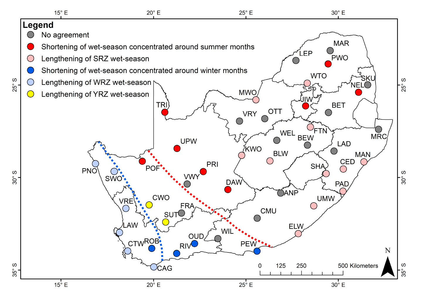
That reconciliation step could be built into the analysis itself, by treating the components as one multivariate object from the start rather than assembling them afterwards.

Refinement three: rank deficiency in the components

Two exact relationships hold by construction:

\[\texttt{length} = \texttt{end} - \texttt{start} + 1 \qquad\qquad \texttt{rate} = \frac{\texttt{total}}{\texttt{raindays}}\]

Eigenvalues of the correlation matrix:

full (7):  3.176  1.759  1.008  0.724  0.305  0.027  0.000
core (4):  2.465  0.999  0.371  0.165

The smallest root is zero, not small. Seven components span six dimensions exactly.

So the 322 tests draw on six degrees of freedom per station, not seven. No individual result is invalidated, but it suggests there is more room in a multiple-testing correction than the raw count of 322 alone would imply.

This is the strongest technical argument in the talk and it belongs here, at the end of the univariate section, as the thing that motivates everything after it.

What a multivariate treatment offers

A claim like “a shift from winter-rainfall towards year-round conditions” becomes a trajectory, not a set of \(p\)-values needing subsequent alignment.

2. moveEZ

The problem the package solves

Data on \(n\) samples and \(p\) continuous variables, plus one variable representing time. Time need not be chronological: it can be an algorithmic iteration, an experimental stage, or any ordered index.

The natural approach is one biplot per level of the time variable. With thirty levels this produces thirty biplots and no way to read them.

moveEZ animates a single biplot across the levels instead.

Built on biplotEZ objects. On CRAN, version 1.3.0. Ganey & Nienkemper-Swanepoel.

Two conceptual frameworks

Fixed variable frame

moveplot()

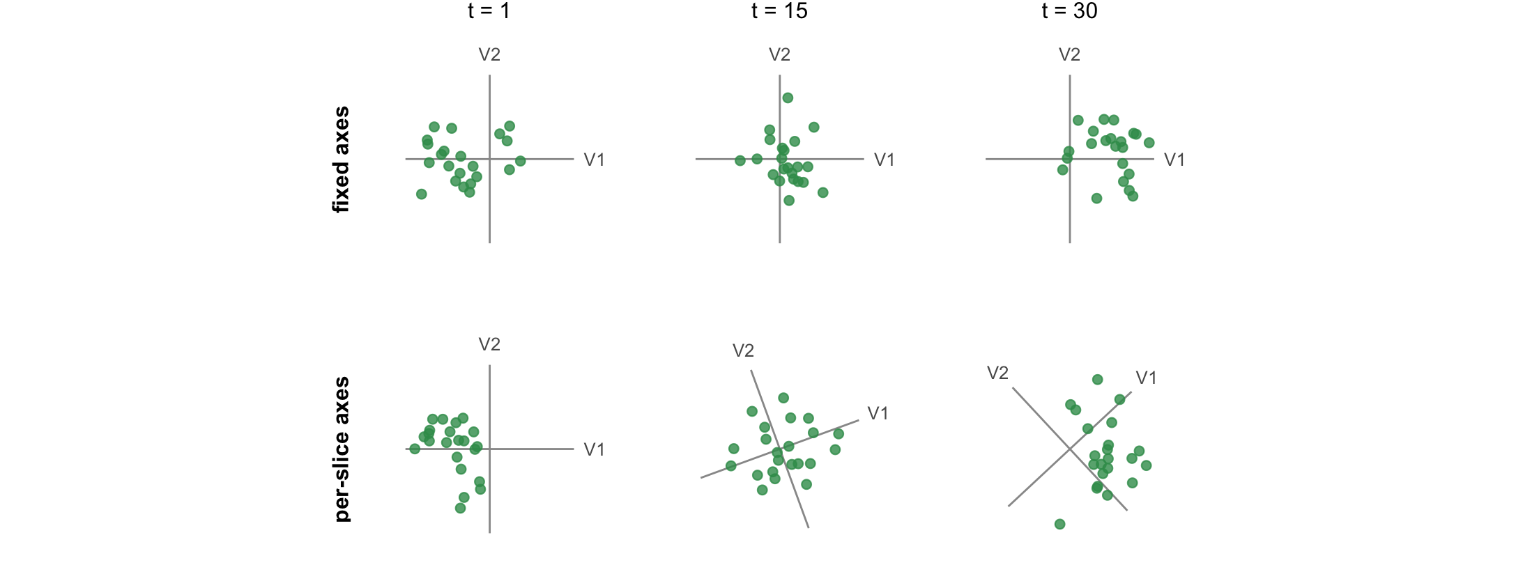
One biplot is constructed on the full dataset \(\mathbf{X}\). The animation slices the observations by the time variable.

Variable axes stay fixed. Only sample points move.

Dynamic frame

moveplot2(), moveplot3()

A separate biplot per time slice. Both sample points and variable axes evolve.

Continuity across levels is maintained by Procrustes alignment and reflection.

The choice is not only graphical between the frameworks, it also determines what movement on the screen means.

What movement means

Under fixed axes, movement on screen is movement in the data. Under per-slice axes, movement mixes real change with a moving frame of reference.

The grammar

moveEZ extends the biplotEZ pipe:

library(biplotEZ)
library(moveEZ)

bp_ann <- biplot(ad, scaled = TRUE) |>
          PCA() 

 
bp_ann |> moveplot(time.var = "year", 
                   group.var = "zone",
                   hulls = FALSE, 
                   move = TRUE, 
                   label.vars = "zone")

move = TRUE animates through gganimate

move = FALSE returns static faceted panels instead.

Alignment and evaluation

results <- bp_ann |>
  moveplot3(time.var = "year", 
                   group.var = "zone",
                   hulls = FALSE, 
                   move = TRUE, 
                   target = NULL) |>
  evaluation()

Generalised orthogonal Procrustes analysis compares each testee configuration against a target. With target = NULL the target is estimated from the configurations themselves.

The five comparison measures

Measure	Reads on
Procrustes Statistic (PS)	overall residual after optimal alignment
Congruence Coefficient (CC)	similarity of configurations, scale free
Absolute Mean Bias (AMB)	typical size of displacement
Mean Bias (MB)	systematic directional displacement
Root Mean Squared Bias (RMSB)	displacement penalising large errors

results$eval.list  
results$fit.plot 
results$bias.plot

These are the package’s answer to a question the animation itself cannot settle: is what I am seeing real, or is it the frame moving?

3. Application

Global biplot

Overall quality 0.866

Axis predictivity

Variable
length	0.938
raindays	0.908
total	0.852
score	0.766

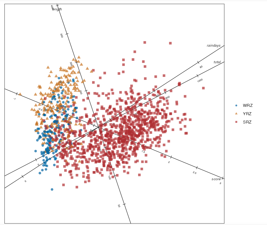
All station-year points in one biplot.

The space is two-dimensional and interpretable

Variable	PC1	PC2
length	-0.288	0.857
total	0.558	0.290
raindays	0.561	0.364
score	0.539	-0.221

Total 86.6%

PC1 is amount and character. Wetter, more rain days, more strongly summer-rainfall. Three variables load almost identically.

PC2 is length of rainfall season. Lower - shorter season, larger - longer season.

The components organise into two largely independent aspects. This is exactly the amount against length distinction the source paper makes qualitatively when it notes that length can change without totals changing.

PCA in the fixed variable frame

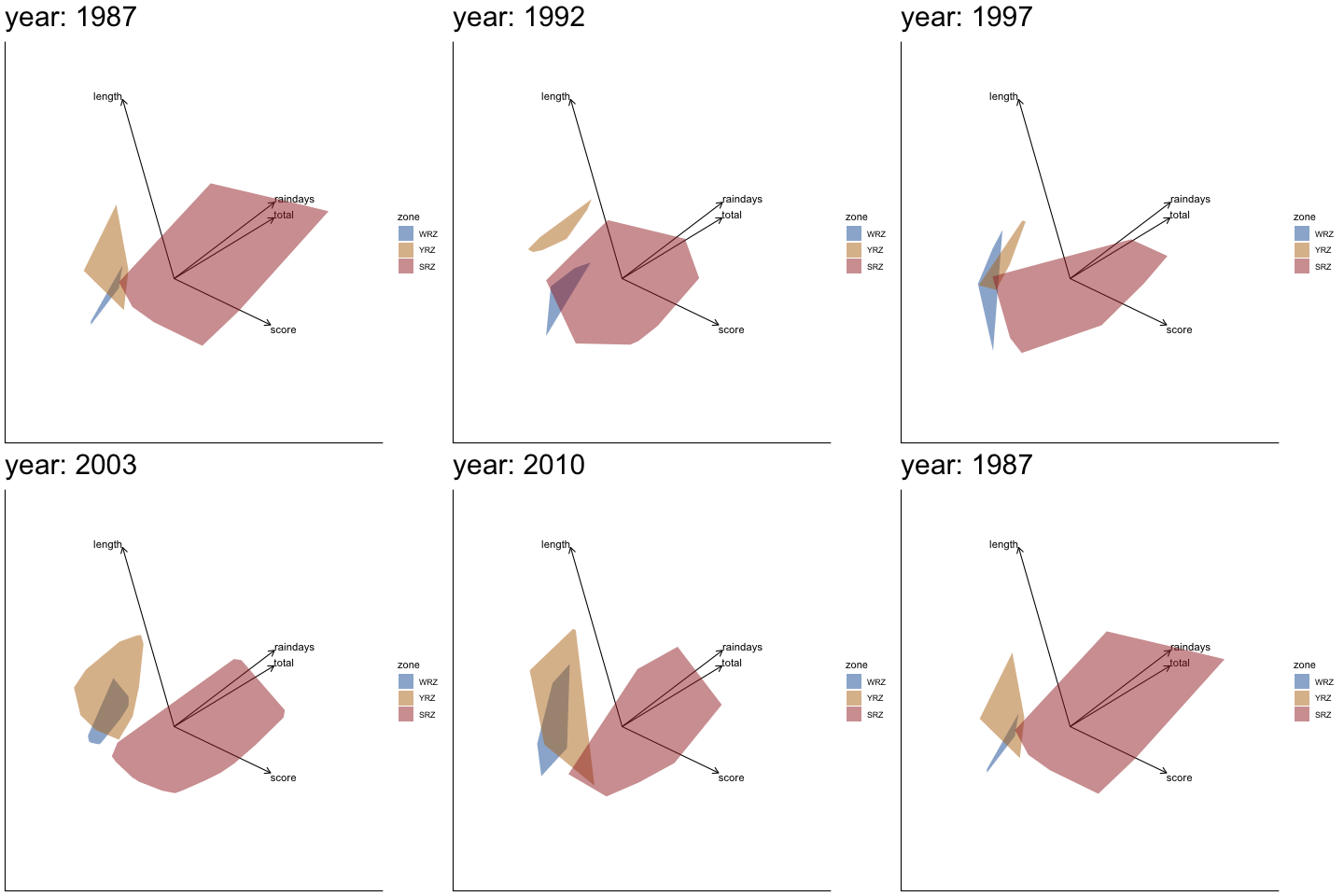
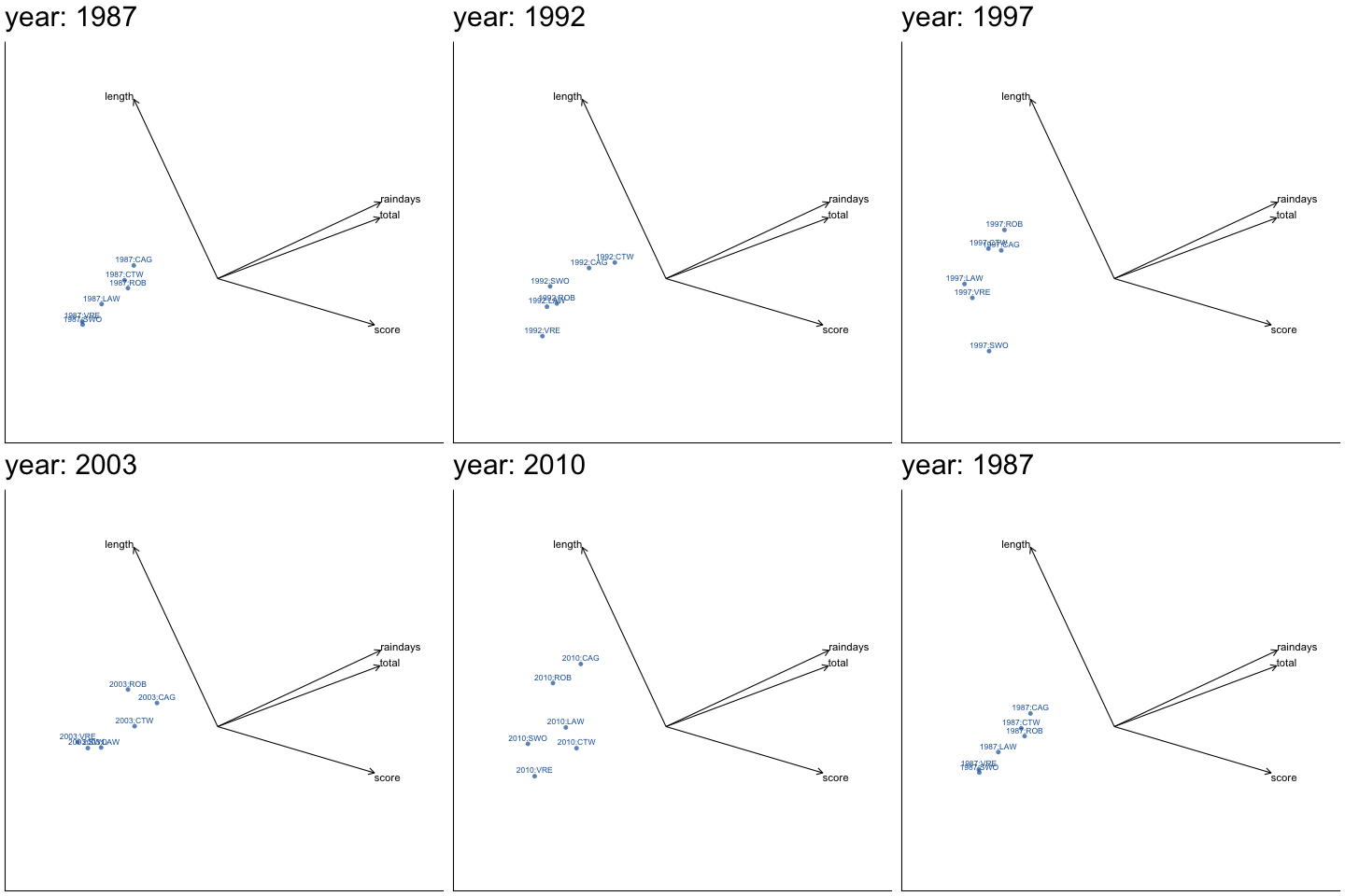
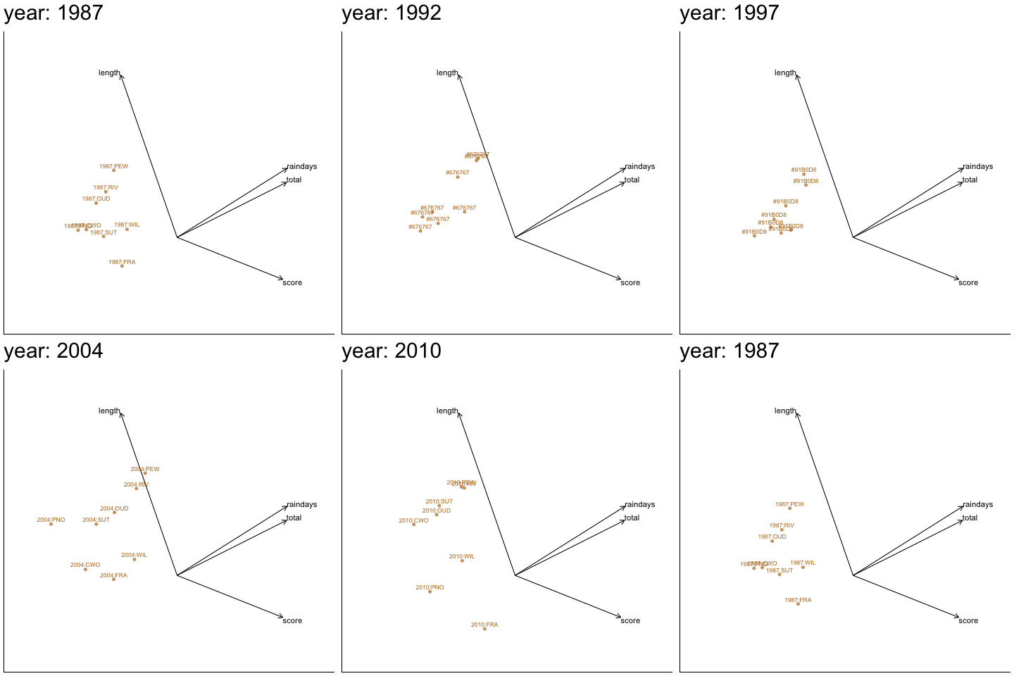
Using the function moveplot():

Display per zone

Only samples move in this framework. We should ask the question on whether the variable relationships are changing over time?

PCA with a dynamic frame

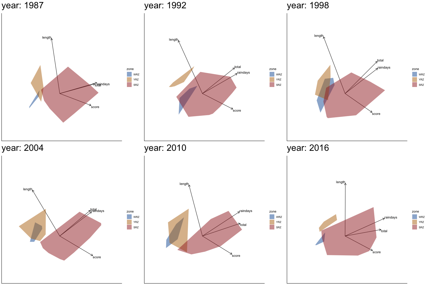
Using the function moveplot3():

Compare against the fixed-axis panel: sharp disagreement would mean the covariance structure is changing, not just the station positions.

The question the two frameworks pose

Fixed axes and PCA per-slice axes can only disagree if the covariance structure of seasonality is itself changing over time.

Stations drifting within a stable space is one claim.

The space itself deforming is a stronger one, and it is invisible to univariate trend testing, because no single component need show a trend for it to happen.

Two independent diagnostics

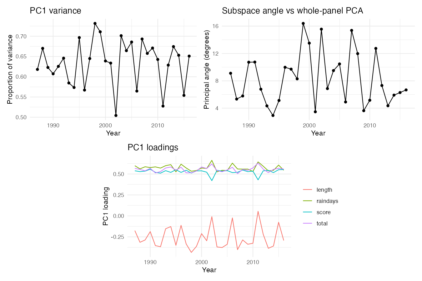
Per-year PCA structure

• proportion of variance on PC1
• loadings of each variable on PC1
• principal angle between that year’s plane and the whole-panel plane

Each tested for monotonic drift against year by Spearman correlation.

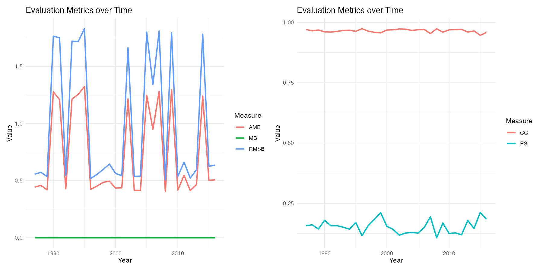
Procrustes measures from moveplot3()

The five comparison measures, per slice, against the GPA target.

A second and independent read on the same question.

Per-slice PCA check

Spearman drift test

Quantity	ρ	p	sig
pc1_var	0.101	0.593	–
angle_deg	-0.031	0.871	–
length_load1	-0.046	0.809	–
total_load1	0.099	0.601	–
raindays_load1	-0.209	0.266	–
score_load1	0.085	0.655	–

No significant correlation, so the variables are not evolving over time.

Fit and bias measures

A useful result

The apparent divergence was per-slice instability at 46 stations per year, not a changing covariance structure.

For the climate question: the seasonality space is stable over 1987 to 2016. Stations move within it; it does not deform under them.

For moveEZ: report on the fixed variable frame as primary, treat dynamic frame as a robustness check.

What the joint view adds

• Redundancy is visible. Seven components, four dimensions
• The amount and timing split is empirical, not asserted.
• Zone separation persists throughout the period rather than being tested station by station.
• The stability result exists. No arrangement of 322 univariate tests could have produced it, because it is a statement about the relationships between components rather than about any one of them.

4. Are the sample positions drifting, and how strongly?

Rationale

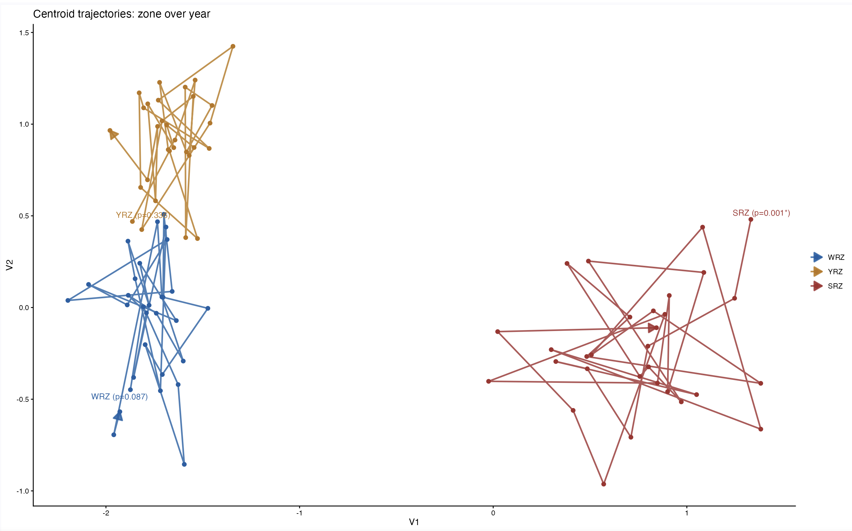
Tests whether a group (rainfall zone or station) is drifting over time, or just sitting there noisily.

• One MV test: PERMANOVA on the full raw station-year data (all 4 metrics) run per group (zone or per station).
• One picture: the group’s centroid path in the biplot space, labelled with that test’s p-value.
• Permutation is restricted within stations, so repeated years from one station aren’t treated as independent evidence.

Zone positions

Station positions

5. To conclude

What has been claimed

• Seven components span six dimensions exactly.
• The space is two-dimensional, splitting into amount and length.
• The covariance structure is stable over 1987 to 2016.
• Inferential statements are made about zone and station trajectories.

Next

• Check with my climate scientist that this all makes sense :)
• Phase 3: extend to 1981 to 2025 and to the full 0.05 degree grid, moving from 46 stations to a spatial field
• Feed the diagnostics back into moveEZ

Changes in rainfall seasonality viewed as a coherent multivariate movement, rather than as a collection of disconnected trend tests.

Thank you

Raeesa Ganey

School of Statistics and Actuarial Science University of the Witwatersrand

install.packages("moveEZ")

https://raeesaganey91.github.io/Wits-Seminar-Slides

https://muvisu.github.io/moveEZ/

Slides made in Quarto. Raindrops on first slide were generated by AI.

This work is licensed under a Creative Commons Attribution-ShareAlike 4.0 International License.

Appendix

References

Ganey, R. & Nienkemper-Swanepoel, J. (2026). moveEZ: An R Package for Animated Biplots. arXiv:2605.22284.

Ganey, R. & Nienkemper-Swanepoel, J. (2025). moveEZ: Animated Biplots. R package version 1.3.0.

Lubbe, S., le Roux, N., Nienkemper-Swanepoel, J., Ganey, R., Buys, R., Adams, Z. & Manefeldt, P. (2024). biplotEZ: EZ-to-Use Biplots. R package version 2.2.

Roffe, S.J., Fitchett, J.M. & Curtis, C.J. (2021). Investigating changes in rainfall seasonality across South Africa. International Journal of Climatology.

Roffe, S.J., Fitchett, J.M. & Curtis, C.J. (2020). Quantifying rainfall seasonality across South Africa on the basis of a percentile metric. Theoretical and Applied Climatology.

Gower, J.C., Lubbe, S. & le Roux, N.J. (2011). Understanding Biplots. Wiley.